A little SF vignette

Canada has these laws that require a certain fraction of the music that is broadcast to be Canadian. This caused a certain amount of screaming from radio stations, but I have this feeling that it actually works, that Canada as a result produces disproportionally more music, and more original music. I don't know about that (how would you quantify it?), but this band — You Say Party — is Canadian.

arXiv gleanings

I try to keep an eye on arxiv.org because interesting new pulsar papers generally appear there first. But there are often abstracts that catch my eye, whether because they have neat ideas, because they talk about neat object, or because they just seem peculiar. This week's batch had a few of each.

How tempo2 does its fitting

Pulsars can be difficult objects to study: for example, their radio pulses can randomly change in brightness, turn off, turn on, change shape, and we really don't know why. Nevertheless there has been some excellent science done by studying those very radio pulses. The trick has mostly been to simply not care how bright they are or what shape they have and focus on when they arrive. Since this comes from the rotation of the pulsar, this tends to be very regular. After all, for a ball 10 km across, with more mass than the sun, smoothed to within a millimeter by its own gravity, it takes an awful lot to change how fast it's spinning. What's more, time is the quantity we can make the best measurements of - world time standards drift by something like microseconds over decades, which is something like one part in ten to the fourteen. So pulsar timing is a powerful technique, that can measure pulsar positions and distances, spin-down rates and braking indices, and binary orbits. The standard software has been tempo, which is written in FORTRAN and has certain limitations. A new tool has recently appeared, tempo2, written in C++ and boasting good handling of timing effects down to the nanosecond level. Unfortunately the documentation on this tool is so far somewhat limited, so I've been figuring out how it works. I'd like to describe it, as best I understand it, here. This particular post will talk about how a timing solution is fit to a set of pulse arrival times.

Millisecond pulsar X-rays

Neutron stars are so tiny and so dense that the natural temperature scale for them has them glowing in the X-rays. What's more, they serve as powerful accelerators of electrons, which then naturally produce X-rays. So it turns out that X-ray telescopes provide a very interesting view of pulsars. In light of this, when we discovered my pet source, J1023, we took an X-ray observation of it. It's taken us considerable time to analyze the results and put together a paper describing them, but I think the result will be a valuable contribution to the literature. (More importantly for me, it should make a chapter of my PhD thesis.) The result is the cumbersomely-named "X-ray Variability and Evidence for Pulsations from the Unique Radio Pulsar/X-ray Binary Transition Object FIRST J102347.6+003841".

Much of the paper is devoted to details of data analysis, which I will spare you. But I think the gist is interesting, and not too hard to summarize. 

Ignition!

Recently, via Derek Lowe's In The Pipeline, I came across the book Ignition!, by John D. Clark. It's the story of the development of liquid rocket fuels, told by a man who was head of one of the programs. Even if you don't know much chemistry — I don't — the book makes a fascinating read. The image on the left is the first page you see when you open the book, and the image below is the second.

Ergo Proxy

As is obvious to regular readers of this blog, I read a lot of science fiction. I also enjoy science fiction movies and TV shows, but they're generally much harder to find. Or at least, ones I like are. But I came across an enjoyable new series recently: Ergo Proxy. It's a cyberpunk anime with a female protagonist that I came to rather like in spite of her cold and sometimes difficult personality. The series is obviously some sort of cousin to Ghost in the Shell (albeit without some of Shirow's particular obsessions) and Serial Experiments Lain (though thankfully free of schoolgirls). On the Western side, I suppose I'd compare it to The Matrix (or maybe the similar-but-better The Thirteenth Floor) and The Prisoner. 

As those analogies suggest, the series is sometimes a little heavy on the symbolism, mystery, and spouting of philosophy, but that's all part of the cyberpunk tradition, and this series carries it off well. I enjoy the visual style as well, though there are a few moments where the animation is a little off. The soundtrack is the kind of music I listen to anyway, which helps. I usually prefer subtitles to dubbed audio, but for this show the dub is better written and well-acted. All together a fun experience. 


[Edit: you can watch the whole thing online.]

Reporting FAIL

There's currently an item in the news about a British boy who managed to damage his eyesight with a "laser pointer". The news articles generally imply that any laser pointer is a lurking risk to your eyesight ready to blind you with a single incautious glance. But there are the ordinary 1-5 mW laser pointers you can buy in dollar stores, and then there are the pocket lasers you can buy online that have powers up to 500 mW and that can burn a hole in a credit card. If this kid managed to damage his eye with the former, well, that's surprising and alarming. But the articles don't describe the laser at all, beyond the fact that he ordered it on the internet. If you go to the original one in the British Medical Journal, though, you still don't get the power rating, but you find out that it was "high-powered", i.e. almost certainly one of the high-power ones you can get online. Of course you can damage your eyes with these; I strongly doubt it would be possible to get one without being made aware of the danger. What's more, the high-power ones are already arguably illegal in many places, not that that stops online companies from shipping them there.

The key point I'm getting at is that all the media coverage is missing the essential information that this is not a normal laser pointer, and that those are basically not dangerous.

[Edit: I emailed the corresponding author of the BMJ piece. Unfortunately the boy's guardian destroyed the laser before the doctor could see it, but the doctor is certain that it was one of the high-powered lasers I describe above. It's too bad none of the reporters bothered to check that detail, but I guess it doesn't make good copy.]

Virtual idol

Years ago, I'm not sure when or where, I saw the anime Macross Plus, which is about a pop star who is entirely a computer program that sings, but who has fans as devoted as any present-day pop star. Anime being anime, there was of course a whole plot line about her AI going rogue (plus giant robots of course), but I remember thinking "how weird, a pop star who doesn't exactly exist". Well, technology progresses, and sure enough, we have one now.

Laser rifles

Laser rifles have been a staple of science fiction for years, though now that cheap harmless (or nearly) lasers are everywhere writers are moving to other buzzwords. But I had no idea that anyone had come up with a more-or-less workable design until I stumbled across the "Stavatti SF-1" and "TIS-1".

(More below the jump.)

CASCA 2010 compact objects session 1

Orbital eccentricity in numerical simulations of binary black holes (Harald P. Pfeiffer)


Eccentricity in black-hole binaries is radiated away faster than the semi-major axis, so that they become circular fairly rapidly. Thus, for example, when a binary makes its way into the LIGO band the eccentricity is down around 10^-6. For numerical GR this means you have to be able to measure - for that matter, define - eccentricity, and you need to be able to produce near-zero eccentricities. To define it, you often construct some function that measures deviation from a circular inspiral, but this is difficult because of (among other things) coordinate dependence. It turns out it works better to define eccentricity in terms of its  gravitational wave effects. You also have to work on periastron advance (for which third-order post-Newtonian models are not good enough). How is very low eccentricity achieved? The problem is in constructing your initial data: coordinate location, sizes, velocities; these need to satisfy complicated PDEs to satisfy the constraints, and it's not clear what goal values you should choose to get circular orbits. The approach is to simulate a few orbits, then fix the initial condition as if it were Newtonian; this roughly works, so you iterate the process until you get a nice low eccentricity. When you go to precessing binaries (i.e. rotating black holes) spin-orbit coupling complicates your life, but you can still extract an eccentricity measurement and initial condition corrections.

Rayachaudhuri's Equation in Regge Calculus (Parandis Khavari)


These equations are important in the proof of singularity theorems, lensing, collapse, and cracking under self-gravity. They concern expansion and shear of fluids in self-gravitation. Absent vorticity they imply collapse into a singularity in a finite amount of time. Regge calculus is finite-element GR that fixes flat geometry within simplices; curvature is concentrated on n-2-dimensional sub-simplices ("bones") and can be described by the deficit angle. Geodesics in the Regge calculus are straight lines within simplices; where they meet faces, the angle on the entrance edge matches the angle on the exit edge, but it's a little tricky since there's no unique way to assign the deficit angle to the n-1 simplices around a particular bone. This work is about expansion of geodesics in (2+1)-dimensions. She obtains expressions for shear and expansion of lensing. Remaining problems include that Rayachaudhuri's equation has no unique discrete representation.

Numerical simulations of precessing binary black holes (Abdul Mroue)


Gravitational wave detection will only be possible if we have accurate banks of template gravitational waveforms. The three main categories are inspiral, merger, and ringdown. To build these templates we need some combination of post-Newtonian models and numerical relativity. We expect an event in the LIGO range at a rate <1/year, but advanced LIGO should have ~0.5/day. So building a template bank is crucial. The parameter space (for zero eccentricity) is given by the mass ratio and the two spins. A 15-orbit binary takes ~10^5 CPU-hours (plus a great number of grad student-hours). Less than 100 waveforms are available from all groups worldwide. So far very little work has been done on systems with generic spins. The spin has very significant effects on the system evolution. This work has two major approaches: make BBH runs easier (i.e. reduce the person-hours) by automating the initial setup and transition between regimes, and make BBH runs faster, primarily by making their simulation code run on GPU supercomputers (possibly an order of magnitude speedup). Currently running on his desktop's GPU.

Questions: Do we expect spin-orbit alignment? Maybe; what happens in the final orbits is totally unclear. [No comment on whether binary evolution is likely to produce aligned binary systems.]

Modelling Gravitational Lens Systems with Genetic Algorithms and Particle Swarm Methods (Adam Rogers)


Lensing has been observed on many cosmological structures; it's interesting because on the one hand it depends on the mass of the lens, and on the other hand it provides an important magnification effect. The goal of this research is to try to reconstruct the un-lensed image of the source. They assume a thin lens. The lensing equation is clearly nonlinear, as shown by multiple lensing. Rather than solve a complicated nonlinear equation, one can simply raytrace past a lens shape. One can combine this information into a mapping matrix; in this formalism, finding the source pixel intensities is a linear least-squares problem. Unfortunately the matrix sizes are comparable to the number of pixels [so you need sparsity], so you need to use a small PSF, i.e. optical data. With some cleverness one can reformulate the problem into a deconvolution problem that never needs to construct the huge matrices. On simulated data it's quite effective at recovering even highly distorted images when you know the lens parameters. Finding the lens parameters requires a fitting procedure, for which he's using genetic algorithms and particle swarms. Particle swarm optimizers attract each particle to its local best and the global best according to a spring force. Of the two the particle swarm optimizer is a little faster, while the GA is much more thorough in searching the parameter space (e.g. local loses one of the two 180-degree options for ellipse orientation).

Questions: Have you applied your models to real data? Yes, but it's old data that's already been partially processed. What is he optimizing? "chi-squared between the model and the data"

New properties od teh 35-day cycle of Hercules X-1 (Denis Leahy)


RXTE ASM data of Her X-1, plus PCA data when available. Her X-1 is 6.6 kpc and high galactic latitude; it's a neutron star with a 2.5 Msun A7 companion. Over 35 days (many binary orbits) you get brightness variations. One model is a twisted disk that occults the NS; its shadow on the companion star changes on the same cycle, which explains the optical variations. ASM data shows that the cycle length varies substantially - 34-38 days - and this variation is correlated with the flux. The turn-on appears to occur uniformly in orbital phase. They have 1.58 Ms of PCA data in total. One idea for explaining some of the irregularities is that the impact point on the disk is not the outer edge, since it's not flat; other models include an uneven disk surface or blobs in the accretion stream, but these don't match the data well.

Questions: Why is the disk twisted? Heating by the central source  produces a torque that increases as the disk gets out-of-plane up to the point where it starts shadowing itself.

CASCA 2010: Stars 3 session

Variable stars in the Hyades Cluster (Jayme Derrah)

To establish distance scales you need to measure variable stars at known distances; the Hyades cluster is the closest open cluster to the Earth. Unfortunately it's just out of range for accurate parallax measurements, so distances are measured using the "convergent point method". Variable stars of interest re eclipsing binaries and pulsational variables (though few new examples of the latter are expected). The project uses the Baker-Nunn patrol camera, which has a large enough field of view to include the whole cluster and reaches a limiting magnitude of 19.5 in two minutes; on the other hand there's only one filter, a light pollution blocker. Follow-up of discovered variables will use B and V.

Type 1A Supernova Progenitor Diversity (Ashley J. Ruiter)

Sub-Chandrasekhar-mass WDs should be looked at as SN1A progenitors. SN1A light curves are driven by the amount of nickel produced, so we can use them as standard candles almost without any idea of what the progenitors look like. Theories are CO WD mergers and CO WD collapse triggered by companion Roche lobe overflow. Simulations predict that the former ought to produce NSes instead, while models (including this work) have difficulty producing enough of the latter. In particular, she built a population synthesis code and found an order of magnitude too few overflow models. The idea is that perhaps allowing sub-Chandrasekhar-mass collapse can help. More detailed models, in particular using helium accretion, allow collapse to occur with 0.8-0.9 Msun: you get detonation in a shell of accreted helium which triggers the explosion. She built simulated light curves based on such explosions and found reasonable agreement with observed light curves [but how hard is this, if nickel mass is all you see?]. From a population synthesis point of view, though, they do provide enough. It's also theoretically nice because it explains the observed variety in light curves: it's a function of mass at collapse.

Questions: Where do these helium-rich companions come from? Many are He white dwarfs, which arise naturally in such binaries (lost their hydrogen through Roche lobe overflow). What's that blue line on the graph? It turns out if you start with 0.9 Msun WDs the merger scenario looks a little more plausible. What assumptions go into the pop. synth? Standard IMF, etc. Where does the mass go during binary evolution? Eddington-limited transfer, so probably outflows.

Tau Sco: The Discovery of the Clones (Veronique Petit)

Part of the MiMeS (Magnetic Field in Massive Star) collaboration. There ~35 known magnetic OB stars (i.e. B directly detected, which is hard), but it has long been suspected that B is ubiquitous in massive stars. ("Magnetic fields are to astrophysics as sex is to psychology." - someone) These stars are short-lived but important, and the key complicating parameters are rotation and mass loss; we expect B to substantially affect the wind (as it does in the Sun). Tau Sco, a B 0.5 V star, is the focus of this talk. We can measure B by the Zeeman effect, i.e. circular polarization across a spectral line. If you sample the stellar rotation, you can actually produce B maps. Unlike all other massive magnetic stars which have roughly dipolar fields, tau Sco's field is complex and multipolar. Studies of the wind using UV line profiles show strange inconsistencies between different line traces; there seems to be some correlation between the UV variability as a function of stellar rotation and the B. It's natural to assume that the wind anomalies arise from the complexity of B, but it was hard to test until their recent discovery of two "clones" that have similar wind anomalies and slow rotation. ESPADON shows that these stars are magnetic; sadly it has not yet been possible to sample the stellar rotation densely enough to map the magnetic field. Preliminarily, though, a dipole model suggests that surface B is roughly equal to that of tau Sco. 

Questions: Have people measured this supposed correlation between B and the wind? Yes, but it doesn't really predict tau Sco. How strong are these Bs? ~500 G. Does B of tau Sco vary with time, particularly in flares? We don't know, they had to assume it depended only on rotation. Could you use the Bayesian inference to estimate non-dipolar fields? There's too much uncertainty when you don't know about the stellar rotation.

Tracing Wolf-Rayet wind structures (Alexandre David-Uraz)

This work focuses on WR113. WR stars have very high mass loss rates, high enough that radiation pressure alone can't explain it; we need to understand the physics of clumping. WR113 = CV Ser is a binary system in which the companion can often be seen through the WR wind. It's a double-line binary, so they can in principle get a decent picture of the orbit, but so far the spectrum has been too messy. Once this is accomplished, they should be able to separate the two spectra quite well - average everything in the WR frame, then subtract this and switch to the companion's frame, then back and forth. In any case, the "eclipse" is of depth ~0.6 mag - well, in Lamontagne et al. from the 90s; in a 1963 paper the eclipse seems variable (0.1 mag sometimes and 0.6 mag), and in 1970 they didn't see an eclipse at all. MOST sees a shallow eclipse but variable - in fact, two successive eclipses differ very substantially. The real focus of the research is random variations due to clumping, and indeed they see both photometric and spectroscopic evidence for clumping. There's also the issue of a colliding-wind shock, which shows up in the lines (in particular there's streaming along the shock); with luck this should help establish system geometry. The next step is Fourier analysis for pulsations in star or wind, and wavelet analysis for random clumping. The goal is to link these to spectroscopic data and constrain the clumping.  

Questions: This is a complicated system; is there evidence for an accretion disk? Unclear, but the colliding winds suggest not. Is this the only eclipsing WR star? No, there are others. 

Limb-Darkening and Stellar Atmospheres (Hilding Neilson)

Limb darkening is particularly interesting these days as observations become more constraining. They affect planet parameters inferred from transits (and fitting can constrain limb darkening). Optical interferometry can directly measure it, and microlensing can help as well. Limb darkening tells you something about conditions in stellar atmospheres; Schwarzschild used solar eclipse observations to show that the solar atmosphere is in radiative rather than adiabatic equilibrium. Traditionally, though, people just use empirical limb darkening laws that are pretty crummy; in fact popular parameterizations have fixed points that are more or less independent of the parameters, and fit observations rather badly. The fixed point arises because the models the empirical laws are based on all make the Eddington approximation. Spherical symmetry rather than plane-parallel atmospheres helps spread the fixed point out. Detailed modelling suggests that the true value at the fixed point probes atmosphere physics. Observations suggest that you can make these inference even with the wrong models.

CASCA 2010: planets session

NIR from hot Jupiters (Bryce Croll):

Hot Jupiters are tidally locked, and one expects their properties to depend on the amount of heating. He tested this with four known hot Jupiters. To get good photometry, he used WIRCAM out-of-focus (!). This lets them detect the thermal emission from hot Jupiters (millimagnitudes). "Hot" and "hotter" distribute heat very effectively, though "hotter" shows abnormally low H-band emission; maybe an absorber? "Even hotter", on the other hand, doesn't distribute heat very effectively. "Hottest" shows redistribution within the hot side but not between sides, plus evidence for a thermal emission deep in the atmosphere.  Many more CFHT observations are planned.

Music of the Spheres: Results from the Kepler Mission (Jason Rowe):


Kepler's a 1m space telescope designed for steady monitoring of a fixed field of 100000 stars, looking for exoplanets and asteroseismology. CCDs were placed so that the brightest stars fall into the gaps. Kepler's bandpass is more or less white light (400-900 nm). Measurements as good as one part per million for  many stars; Kepler's working very well. The parameters you fit directly include stellar density. The smallest planet so far is ~Neptune-sized, but some secondary transit measurements show you could detect a terrestrial transit. In asteroseismology they should get p-modes for every star brighter than ~12 mag. Also some weirdos like helium white dwarf companions, for which radial velocity followup has begun. Apparently Kepler also has Guest Observers and Target of Opportunity arrangements.   Quite what this means I'm not sure, since the instrument isn't pointed.

In questions, they do have lots of earthlike transit candidates - but they get lots of false positives from photometry alone, let alone grazing transits by bigger objects.

SPI or Spin-up? An UV Investigation of Activity on Exoplanet Host Stars (Evgenya L Shkolnik)

"SPI" is "star-planet interaction", meaning magnetic. Spin-up is tidal effects of the planet on their stars. These should occur since the planets are so close to their stars. Both should show up as increased stellar activity (hence the UV). Looking at X-ray data, there's debate about whether this is observed. She used GALEX (175-275 nm). GALEX sees almost every exoplanet host star (that's in its field of view). Given 135 GALEX detections, start with close-in planets seem to be ~2x brighter. (Planet distance is a bimodal distribution, so there's a natural dividing line here; we think it's migrated versus not migrated.) A few transiting systems have been observed to have abnormally rapidly rotating stars; if this is a general phenomenon, gyrochronology goes out the window. The exceptions, stars that aren't active in spite of close-in planets may be explicable in terms of some scattering models but not others, and in fact the exceptions are more eccentric, consistent with the potentially recent scattering models.

Super-Earth Transit Search with the MOST Space Telescope (Diana Dragomir)


Start with radial velocity candidates from HARPS; F, G, K with 2-20 Mearth planets. MOST watches during the transit window. Key transit parameters are period, phase, duration, and depth. Diana's idea is to use Bayesian methods to fit the model, which is feasible mostly because the HARPS candidates provide a drastically reduced parameter space. (Ew! She uses JDs!) This parameter space needs to be very finely sampled to avoid underestimating the depth. (She's using grid sampling rather than MCMC because of the small low-dimensional parameter space.)

Ultra-Wide Trans-Neptunian Binaries (Alex H. Parker)

You classify TNOs based on their resonance with Neptune: the plutinos, for example are roughly 3:2 times the period. The big question is how the TNOs got there, since they haven't had time to form in situ. One answer is that as the giant planets moved out to their current positions they scattered the planetoids out into the outer solar system. This talk is about binaries; binaries are present throughout the solar system. Binary asteroids are different, as they tend to have large mass ratios and tight circular orbits, suggesting a collisional origin. The TNOs have lots of binaries, with a wide range of eccentricities and often modest mass ratios. These binaries are interesting observationally because you get mass measurements. Wide binaries are resolved with Gemini, and they're so delicate you can test dynamical ideas with them. Their formation mechanism is debated, maybe three-body exchanges, maybe temporary capture into chaotic orbits, but the mutual orbit distribution should allow them to be distinguished. His sample is >0.5'' apart and mags differing by <1.5. Typicallt separations ~1'' and mags ~24. Terrestrial parallax allows measurement of things like the direction of the orbital axis. The observed distribution doesn't really fit with either formation model. You can also use these to look at the number of ~1km objects in the Kuiper belt, since these objects will eventually break up such a system. These small objects  can't be made through accretion or collision, they have to be primordial.

HST Compositional Survey of Faint Kuiper Belt Objects (Wesley C. Fraser)


The idea is to look at chemical gradients in the protoplanetary disk; this is closely related to understanding their scattering history, which is what dominates their current dynamics. Compositionally, only the biggest can retain methane (as it evaporates on a timescale of thousands of years). The fainter ones you don't get much in the way of lines, so the data is mostly colour (some are neutral, some are quite red). In the IR you do see deep water ice on certain objects ("family members" in resonances?) but not on others. It's a little puzzling what these objects are actually made of. Fortunately WFPC-3 is almost ideal for this work, with filters for water ice, methane, and a couple of useful narrow-line filters. The colors show evidence of a mix of water ice and some red gunk in varying proportions. Centaurs, objects that have been scattered further into the solar system show evidence for solar processing. Other objects are more mysterious.

Searching for Main-Belt Comets Using the CFHT: Final Results (Alyssa Gilbert)


Main-belt comets reside in the asteroid belt but show cometary activity. Their origin is unknown; formed in situ, which would be weird, since we don't expect ice within the orbit of Jupiter, or maybe formed further out and somehow got stuck in the asteroid belt. Only five objects are known, and have been recently found. Small bodies are interesting because they form in different parts of the solar system, and they don't have sesimology or weather, so they provide fairly direct pictures of the structure of the early solar system. To find these objects, she used the CFHT legacy survey data. The cadence is 3 observations in one night followed by another a night later (weather permitting). Automated object selection not terribly effective; visual inspection of 25000 objects worked better and found one. (Somebody has a very high tolerance for boredom...) Unfortunately the object wasn't noticed until a year after the observations, so even though a rough orbit was found the object was lost.  Asteroids activated by collision might produce an appropriate number, but the activity of some of these objects seems to be periodic, which is weird. Capture from the outer solar system should provide too many.

Light echoes

Occasionally some astronomical event — a gamma-ray burst, a supernova, a magnetar flare, or whatever — will go off, lighting up the sky more or less spectacularly and then fading. Normally that's the end of that event, and we're left to wait for the next one. (In particular, this means that if you study this sort of thing, you need to be prepared for one of these things to happen at any time, so that you suddenly need to write target-of-opportunity proposals, analyze data, and release preliminary results in a tearing hurry. This typically happens while you're supposed to be on vacation.) Once in a while, though, we see a peculiar phenomenon called "light echoes".

A "light echo" arises a little like an ordinary (sound) echo: some event happens producing a bright flash (loud noise) and in addition to the light (sound) making its way to you directly, some of the light (sound) goes in a different direction, bounces off something, and makes its way from the other object to you, arriving a little later. From the place I usually stand to watch the summer fireworks competition, you hear the big skyrockets go off, then a second or two later you hear the echo from a nearby building. Of course, on human time and distance scales, the light from the fireworks reaches us instantaneously, so it's obvious that both the original sound and its echo are delayed. In an astronomical setting, we only receive light, and it takes very much longer. But it's still possible to receive a delayed echo, and studying these echoes can be very informative.

(Photo, courtesy of ESA, to the right is X-ray dust echoes around the magnetar 1E 1547.0-5408, one of the objects people in the group here at McGill study. This interesting dust-echo work is from another group, though. The echoes are from a massive X-ray outburst, which we think was caused when the extremely strong internal magnetic field stresses cracked and twisted a piece of its crust; this twisted the external magnetic field, and the twisted magnetic field produced and accelerated massive numbers of electrons and positrons, which blasted out a torrent of X-rays. At least we think that's how it happened; we saw the torrent of X-rays.)

Spuds

From the arxiv: The Potato Radius: a Lower Minimum Size for Dwarf Planets, by Lineweaver and Norman.

This article is kind of neat, not least for the charming way it uses "potato" (and its adjectival variant "potatoid") as a technical term. The point of it is to try to work out how big an object has to be for it to be round.

Ablation

From the arxiv: Momentum Transfer by Laser Ablation of Irregularly Shaped Space Debris, by Liedahl et al.

I don't have a whole lot to say about this one, but how could I ignore a paper about Giant Space Lasers? They're talking about using them to clean some of the junk out of low Earth orbit. While it would take a great deal of power to completely vaporize space junk, all you really need to do is give it enough of a shove (~100-200 m/s) that it starts to dip into the atmosphere (~200 km altitude), where it will slow down and burn up. Just how much of a shove you can get by zapping it with a laser so that some evaporates is not easy to predict, hence the paper.

The particular kind of Giant Space Laser they're talking about is left to some degree unspecified, but it's clear that you want short pulses, so that you get explosive vaporization (gas flow velocity of ~1000 m/s) rather than gentle heating, and they're talking about 10 J pulses (producing 0.1-1 m/s change in velocity for a 1 g target). So it's an awful lot of short powerful pulses. They also mention, in the usual understated scientific way, the possibility of "structural modification" of the debris — that is, the possibility that the bolt or paint flake or whatever will be blown to pieces or bent out of shape by the laser (in addition to the ~10% of the mass that will be outright vaporized). They suggest laboratory experimentation, to which I say, can I help zap random pieces of junk with a high-powered laser and see what happens? Please?

(Photo to the right is of a NASA laser ranging experiment, not actually zapping space debris. Unfortunately.)

Space Race

In honour of Yuri's Night, I'd like to point to this rather nice BBC documentary:

It casts the space race as a personal competition between Sergei Korolyov and Werner von Braun, and is mostly recreations and dramatizations (including the peculiar decision to have the Russians speak English with a Russian accent, except for commands like "Ignition" and "Launch", which the actors could presumably learn and are subtitled). But it's generally well made, and doesn't shy away from either von Braun's Nazi past or the military applications that drove the space race itself: a rocket that could put a man into orbit could also deliver a warhead to a major city, and vice versa. From a public relations point of view, announcing a new milestone in the space race generally went over better than announcing one's ability to more effectively kill millions of people.

Chemistry at home

YouTube user TheHomeScientist (via In The Pipeline) is posting a series of videos about what you can do in a home chemistry lab; as a nice example, there's this beautiful one about the purification of hydrochloric acid:

Isn't this method elegant? No complicated boiling or fumbling around with strong acids; just take advantage of the fact that HCl is a gas.

I think it's great to show people that you can really do chemistry at home. Science is not just the domain of white men in white coats with PhDs. On the other hand, I'm hesitant to get too ecstatic about how "democratic" this is. Not just anyone can afford the time, energy, and space to set up a lab like this.

Parmesan oregano bread

This is a very tasty bread that's rich enough to eat by itself, rather than as a substrate for some more flavourful substance. It also smells wonderful:

• 300 mL water
• 50 mL sugar
• 15 mL oregano
• 250 mL grated parmesan (or romano)
• 5 mL salt
• 750 mL white flour
• 20 mL olive oil
• 10 mL yeast

I brought this to our neutron star discussion group and it was a hit. 

Gallium surface gunge

Gallium, as a safer liquid metal than mercury, has two major drawbacks: the surface rapidly acquires a layer of dull oxides, and when in contact with surfaces it tends to leave a thin layer behind. I've been doing some reading to see if I can work around this problem, and I came across this enjoyable article (which may be behind a paywall).

Digital: A Love Story

For those of us who remember the days of BBSes and 2400-baud modems, Digital: A Love Story has considerable charm. It's a game in a genre — ren'ai — with some conventions that take some getting used to, but it's clever and original enough to be fun even if you weren't using computers in 1988 and haven't played ren'ai before. Recommended.

(It's also in python, using a framework, renpy, that has been a major success.)

Real interbinning

(This is another of my highly-technical "note to self" signal processing posts. I'll put up something less arcane soon.)


The Fourier transform is great for finding periodic signals: you take an FFT and a periodic signal looks like a peak in the output. Well, in an ideal world, that is; you only really get such a neat and tidy peak if the periodic signal is exactly at a Fourier frequency, which happens when it makes exactly an integral number of turns over the course of the data set. If the signal is somewhere between two Fourier frequencies, the power is spread over several Fourier output values. While it's possible to interpolate a very accurate value based on the ~32 nearest values, this can be expensive, and there's a shortcut called "interbinning"; it doesn't reconstruct the phase, but you just take a scaled average of the two neighbouring bins and get a decent approximation to the value at the midpoint between two independent Fourier frequencies.

My problem, for this post, is that the theory is all nicely worked out when going from the time domain to the frequency domain, but I want to do something analogous while going from the frequency domain back to the time domain, if that's possible. (I haven't done a literature search, or even looked very carefully at the frequency-domain interbinning papers; I thought this would be a good exercise for me.)

bash pipes

I've been using UNIX for a very long time, and bash has been my shell for almost all that time, but for the life of me I can never remember how to pipe standard error anywhere. I think my problem is I've never found any logic by which the syntax makes sense. Anyway, it's:

command 2>&1 | less

But if you want to send the standard error and output to a file, it's the other way around:

command > file 2>&1

ISS in the X-band

Pretty Picture: ISS in the X-band - The Planetary Society Blog | The Planetary Society

This spooky-looking image is the international space station as taken by a radar satellite, the German TerraSAR-X.

I actually worked with these radar satellites, though they are now my natural enemies. The basic way they work is very clever, and with appropriate analysis, you can extract things like tiny movements of glaciers from the data.

Glitches and flares

Recently on the arxiv: Searching for X-ray Variability in the Glitching Anomalous X-ray Pulsar 1E 1841-045 in Kes 73, by Zhu and Kaspi.

Pulsars normally spin down very regularly — like clockwork, as the saying goes, and many pulsars spin down as regularly as a good atomic clock. But some pulsars, once in a while, will suddenly start spinning more quickly. This sudden (instantaneous as far as we can measure) spin-up is called a "glitch", and its full explanation remains mysterious. Generally, all we see is that the pulsar is suddenly spinning faster: no heating of the crust, no sudden X-ray emission, no radiative changes at all, just a suddenly-faster pulsar.

Anomalous X-ray pulsars (AXPs) are one kind of "magnetar", pulsars whose magnetic field is so enormous that its decay powers the X-ray emission of the star. They exhibit many peculiar behaviours, and are a major field of study in pulsar research. AXPs will occasionally become much more active for a while: they become much brighter, they emit random blasts of X-rays, and they do other peculiar things. It seems as if they may glitch every time they become active like this. If we want to find some sort of relationship between glitches and these active periods, it would be valuable to know whether an active period happens every time AXPs glitch, or whether AXPs sometimes have "quiet" glitches, like normal pulsars. That's what this paper tries to answer.

Killer radiation

I've been working in the undergraduate labs lately, checking the setups for the undergraduate laboratory project course. The course has any number of interesting projects, like spatial filtering of images using Fourier optics, measurements of the Hall effect, demonstrations of Rutherford scattering (after all, he had his laboratory in the building that is, now that it has been decontaminated, our library), and so on. The setup for the experiment on Compton scattering, pictured to the right, has all sorts of terrifying warning signs all over it, because it necessarily uses a powerful gamma emitter. Just how dangerous is it?

This is not purely a theoretical question, since the head lab technician caught a student looking down the beam at the unshielded source, prompting the numerous warning signs. So just how much harm did that student do themselves?

The source is about 100 millicuries of cesium 137, and emits 661.6 keV gamma radiation. In SI units, that's four billion becquerels (decays per second). But what does this translate to in terms of exposure (measured in sieverts)? This is a more complicated calculation, since the kind of radiation matters, as well as the geometry and time of the exposure.

For the purposes here, though, I'll just point to a list of gamma ray dose constants, which give the exposure rate in rem/hour for a one curie source at a distance of one meter, and note that in these units cesium-137 has a dose constant of about 0.4. So a hundred millicurie source produces roughly 0.04 rem/hour, or 0.4 millisievert per hour.

At this rate, if you stood there and stared into the source for two and a half hours, you'd get Health Canada's recommended yearly radiation limit for the general public. It'd take a hundred and fifty hours to get the limit recommended for people who work with radiation. At two hundred and fifty hours (if that still counts as "acute") you might raise your cancer risk by 0.8%.

All this is to say that while I don't think it's a good idea to look into the source, and certainly not to touch it, and I wouldn't want to work with it every day, the warning signs are perhaps a bit over-emphatic.

Honey oatmeal bread

I think this is my favourite bread machine recipe so far; light and fluffy, a little sweet, and very tasty.

Flops and the FFT

The Fast Fourier Transform is a wonderful family of algorithms that have made whole fields of study possible. They mostly operate by breaking a large problem into some number of equally-sized smaller problems, all the way down to problems of just a few points. As a result, the prime factorization of the number of points can make a large difference in the speed of the calculation. Traditionally, powers of two have been the fastest (or the only) sizes available, so the wisdom has been that if you have a data set whose length is not a power of two, you should pad it to the next larger power of two. It turns out that, at least in some cases, that is a mistake.

For context, I am still thinking about the problem of coherent harmonic summing in pulsar searches. As I worked out before, it's important to have an accurately-interpolated Fourier spectrum, and it turns out that the simplest way to do this is to simply pad the input array before taking its Fourier transform.

For a two-minute observation, we are taking about twelve thousand power measurements per second (yes, this is basically an audio data rate; but it only appears once we have combined all 4096 frequency channels), so the raw data is about 1.48 million data points (the exact length of our observations varies slightly). We need to pad this to eight times its length to get good enough sampling in the frequency domain, so that's about 11.8 million data points. The question is how much more to pad this in order to make the FFT fast.

I'm using FFTW for the Fourier transform, and it has efficient algorithms for powers 2^a3^b5^c7^d. So while I could pad my FFTs to the next power of two (about 16.8 million), I could also pad them to 12 million exactly, or to the smaller value of 11854080, which still factors nicely (2⁸3³5¹7³). I know that those powers of five and seven are not as efficient as those powers of two, but on the other hand, flops are cheap, while increasing the data size by almost a factor of two potentially means an awful lot more memory access (obviously these giant FFTs aren't going to fit in cache, though FFTW is smart enough to arrange the pieces for the best possible cache coherence). So I thought I'd do a comparison.

The results are:

• 16.8 million points: 1.7 s
• 12 million points: 0.8 s
• 11854080 points: 1.0 s

That is, the power of two is the slowest — in fact it took almost twice as long as the nice round decimal number. Trimming the value further, to 11854080, slowed things down again, presumably because the reduction in memory size was minor, but the prime factorization was worse. The upshot of all this is that, at least for large FFTs, padding to the next power of two is not necessarily a good idea.

Moon rot!

Recently on the arxiv: Long-term degradation of optical devices on the moon, Murphy et al. This paper talks about the retroreflectors left on the Moon by the Apollo and Lunokhod missions, and observes that they have dropped in effectiveness by a factor of ten since they were placed. So far from the moon being a hostile but static place, something has been steadily degrading these mirrors.

Among the things the Moon missions left behind were arrays of retroreflectors. Like street signs, bicycle reflectors, or those weird-looking radar octahedra, these take incoming light and beam it back to where it came from. These are useful scientific tools, because you can fire lasers at them and time how long it takes the pulses to come back, in the process measuring the Earth-Moon distance. The current best setup, APOLLO, measures the distance to the nearest millimeter, which lets us test theories of gravity, detect a liquid core to the Moon, and watch the Moon recede from us (well, at 38 mm/year).

The moon is very far away (unlike the International Space Station, which orbits at an altitude of only a hundred kilometers). So when you beam a laser at it, even if you use a telescope to collimate the beam, it's spread over 7 km when it reaches the Moon. Then any imperfection of the retroreflector, or simple diffraction, spreads the return beam over an even larger area (20 km); your telescope picks up as much of the returned light as it can, but APOLLO sends out pulses of 10¹⁷ photons and gets back only about one photon per pulse. These tremendous losses are a challenge, so the authors of this paper (who work on APOLLO) monitor the efficiency of the system.

What they noticed, spurring this paper, was that the efficiency dropped substantially — by a factor of fifteen — near the full Moon. Now, obviously the full Moon is very bright, so background photons make detection more challenging, but it is easy to measure the background and estimate how much harder it makes detection; this effect is far from enough to explain the dip. By itself, a dip at full Moon isn't that exciting; since the Apollo 15 retroreflector is pointed at the Earth, a full Moon is when the Sun is illuminating it nearly face-on, so thermal effects might explain it (and in fact since it works by total internal reflection, it only serves as a reflector out to about 17° from the vertical, while the dip is about that wide, at 30°; the authors don't mention this, so it may be coincidence).

To investigate this dip in efficiency, though, the authors of the paper went back and looked at older observations. In the initial years, lunar laser ranging was done with the 2.7m Macdonald Observatory Smith Telescope. But rather than compete for time on this large telescope, in 1985, the program switched to using smaller, dedicated telescopes. Unfortunately these smaller telescopes couldn't see the reflections near full Moon, so there's no data from 1985 to 2006, when APOLLO went online. But comparing the APOLLO data to the MST data, they find that the dip at full Moon was not present at first, and gradually grew as time went on. What's more, if they looked at the return rate away from full Moon, they found a uniform decay; right now the retroreflectors are returning about a tenth what they did initially.

So what's happening to the retroreflectors? How are they getting worse? It's obviously not rain or wind, the moon being devoid of either, let alone the kinds of organic decay you see here on Earth. As with almost all real science, the authors cannot offer a definitive answer, but they do discuss some possibilities.

First of all it's worth pointing out that the huge drop in efficiency doesn't mean the reflectors are absorbing all that extra energy; they are almost certainly reflecting it but in the wrong direction. They're cube corner reflectors, and if you distort the shape of a cube corner reflector it doesn't reflect light back in quite the same direction it came in. The authors find it would take about 4°C temperature difference across each cube to produce the full-Moon losses they see. So if for some reason the reflectors are now absorbing a small fraction of the blazing unfiltered sun at full Moon and being heated by it, that could explain the dip in effectiveness. But why are these mirrors absorbing more and more of the sunlight?

The authors' most plausible answer, to my eye, is dust. The surface of the Moon is covered with dust, made by thermal weathering of rocks and by micrometeorite impact. This dust does not of course blow around the way terrestrial dust does, and in a vacuum a tiny dust grain should fall as fast as a rock, so it initially seems difficult to explain how much dust could get on top of the reflector. There are micrometeorites, though, and there is an effect I hadn't heard of before: dust particles become electrostatically charged through irradiation and are either levitated or thrown upward in "fountains" by electrostatic repulsion. We think. What we do know is that observations from the lunar surface show the optical effect of dust above the ground. So however this dust gets up there, some of it can plausibly fall on optical equipment left there by astronauts.

A layer of dust on the surface would also naturally explain the general decay in effectiveness even when not being heated by the Sun. So it looks like perhaps things left exposed on the lunar surface get covered with dust fairly rapidly. This I find interesting in its own right, but there are also various plans to build telescopes on the lunar surface, since these would share the advantage of the Hubble space telescope of images undistorted by atmosphere, while being able to rely on gravity to hold things in place, and possibly even being able to be built out of lunar materials. If they rapidly become coated with dust, those plans will have to come up with some scheme for cleaning the optical elements.

Multigrain bread

My second attempt at a multigrain bread in my newly-borrowed bread machine.

Ingredients:

• 250 mL water
• 15 mL olive oil
• 15 mL sunflower seeds
• 15 mL flax seeds
• 15 mL pumpkin seeds
• 15 mL quinoa
• 15 mL millet
• 5 mL salt
• 325 mL bread flour
• 250 mL whole wheat flour
• 30 mL honey
• 10 mL yeast

Incidentally I need to get more containers for all this flour. It used to be something I bought the smallest possible bags of because I never finished it, but with this bread machine I go through a lot.

(That odd-looking lump on the loaf above is a piece of dough that didn't get properly mixed in. This happens from time to time with this bread machine; it actually pauses during the mixing and beeps at you to give you a chance to push any such lumps back into the mix, but I wasn't paying attention to this loaf. Most loaves don't need this extra attention.)

Bread machine

I'm not a great cook; I usually don't have the energy to cook anything interesting, so I tend to fall back to the very simple. (Plus Montreal has zillions of great restaurants, so it doesn't take much excuse to make me go out to eat.) But fresh bread is delicious, so when I visited my parents and they had a bread machine scavenged from the kerb, I was happy to give it a try. I was impressed, but felt like I would probably use it for a little while and then it would sit cluttering up my kitchen. So when some friends mentioned that they had a bread machine they weren't using, I asked if I could borrow it.

I figure, they used it a lot for a month, then got bored of the bread and put it in storage. If I use it for a month and then get bored, well, maybe they'll find someone else to lend it to afterwards. And maybe after a while they'll have a craving for bread again; seems like a fine solution. (Of course, bakeries are a perfectly fine solution too, and indeed I do like to buy a nice Première Moisson baguette from time to time.)

What sold me on a bread machine was not the fine bread it could make — though I did have some nice loaves — but how easy it was to make bread. Now I can have put off going to the grocery store for far too long, so there's no longer anything perishable in the house, but toss five ingredients in the machine, hit a button, and lo and behold, fresh bread:

• 250 mL water
• 60 mL olive oil
• 15 mL sugar
• 5 mL salt
• 750 mL flour
• 8 mL yeast

This uses the "basic" program and produces a medium-size loaf.

There's even a "French" bread recipe that works if I'm out of oil:

• 250 mL water
• 60 mL sugar
• 8 mL salt
• 750 mL flour
• 8 mL yeast

This uses the "French" program, which kneads more and lets it rise longer, and produces a chewier bread with larger bubbles. Since all bread machine loaves are approximately cubical, this doesn't much resemble a baguette (not that that's the only kind of French bread), but it's still pretty good bread.

The biggest problem with the machine is that it takes three hours to make the bread, and about half an hour before the bread is ready it starts smelling delicious.

Blind Zen programming

A recent alarming network problem while trying to observe remotely at Green Bank brought back memories of the age of the 2400 baud modem, when you could often type faster than the system could display your characters. Fortunately I use the text editor vi, which was designed for these conditions. In fact, in this light some of the user interface decisions make a lot more sense.

The most prominent weird UI decision is that the editor has two "modes": insert mode, in which you can actually type text and it goes into your document, and "beep mode" in which the letters on the keyboard all tell the editor to do something (and it beeps if that something doesn't make sense). For example, to move around your document, the keys hjkl move you left down up and right, respectively. Bizarre as it may seem, these keys are on the home row, so if you're doing a great deal of moving around — particularly common when programming, i.e., debugging — this makes a certain sense. (Plus vi users get so hardwired that these become perfectly rational movement keys in video games.) The decision to have an editor-control mode also means that you don't need to press the "control", "alt", or "meta" keys very often, which makes sense since these often didn't work or were inconsistently placed on old UNIX machines. (I spent a while switching between terminals, some of which had "Caps Lock" and "Control" interchanged, and to this day I disable "Caps Lock" on every keyboard I use.)

The use of ordinary (case-sensitive) letter keys for editor commands also means that there's room for lots of editor commands, and they're very quick to use. So, for example, to search forward, you use "/"; "n" takes you to the next match and "N" to the previous. But there's also "f", which searches forward for a single character. While apparently bizarre, when combined with the ability of commands like "delete text" (d) to take an argument, this means you can do "delete up to the next single-quote" with "df'".

All this makes even more sense when it might be seconds from when you type a key to when you see its effect. So if, for example, you're typing along and you realize "hey wait, that 'a' was supposed to be an 'i'", instead of pressing the cursor keys many times and waiting to see where the cursor wound up, you can compose sequences like "Fari$", which will search back to the a, replace it with an i, and return you to the end of the current line. It's a bit like being the blind Zen archer.

All that said, I must make a peace offering to those in the emacs camp: being written not so much later, it offers similarly complex editing functionality, with similarly unusual (but different) UI decisions. I used emacs for years, switched to vi for some reason or other, and have stuck with it through inertia, mostly. (Even in the ubiquitous text boxes on the web I find myself hitting Escape followed by strings of gibberish. I'm not quite hardcore enough to go figure out how to make Firefox use vi as its editing component.)

RFI

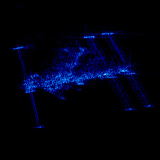
I'm currently involved in another low-frequency pulsar survey with the GBT. This is a pointed survey, so we take two-minute pointings in an array tiling the whole northern part of the sky. This is an incredibly sensitive setup, so we will hopefully find a nice collection of new pulsars. Unfortunately, the same arrangement that makes us sensitive to pulsars makes us sensitive to lightning, electric motors, the local power lines, passing aircraft... all sorts of signals, generally outside our intended piece of sky and/or outside our intended frequency range, but also generally vastly more powerful than the pulsars we're looking for. So dealing with this junk — generically called RFI (Radio Frequency Interference) — is an important part of our survey strategy. My topic today is not so much dealing with the mild RFI we see all the time as dealing with what we see every now and then: a tremendous signal comes booming in, overwhelming everything and ruining the data (as seen on the right).

First of all a brief summary of how our system works: The telescope has a receiver at the primary focus, basically a pair of crossed dipoles. This converts the electromagnetic waves to signals in the wires, where they're amplified, encoded in analog on light and sent down an optical fiber to the control room, where it's converted down to a standard frequency range. This is fed to GUPPI, a so-called "pulsar backend". This instrument does analog-to-digital conversion on the signal then uses a polyphase filterbank to efficiently split it into 4096 channels, then computes the power in each channel; this power is averaged over 81.92 microseconds, after which the set of 4096 powers is dumped to disk.

Pulsars are broadband signals, so we use the widest bandwidth our receiver can handle, about 80 MHz centered near 350 MHz. This gives us the best signal-to-noise from our pulsars, but it also means we can't stick to the few narrow bands reserved for radio astronomy. In fact, the region we're using is allocated for various kinds of radio operation, including "aeronautical radionavigation" around 330 MHz. The GBT is in the National Radio Quiet Zone, so with luck much of this spectrum might be clear, but if aircraft are really using it to navigate there's no keeping them out of our airspace. (And at least once when I've complained of RFI the GBT operator has noticed an airplane passing to the north, for what that's worth.) In any case, there is interference to deal with.

Old radioastronomy systems, in order to get the widest possible bandwidth, quantized the input signal to one bit, or three levels, on initial digitization. This has the serious drawback that any small change in the signal levels causes the digitizer to overload or underflow, trashing the output. Newer backends improve on this by using 8-bit digitization, so that you have more than twenty decibels difference between underflow and overflow; it also helps that they are sampling a wider bandwidth, so that it takes more power to substantially change the levels. So generally, when a noise signal is picked up by GUPPI, it is narrowband and produces excess power in one channel. But the polyphase filterbank is good at keeping it from spilling into neigbouring channels (much better than a simple FFT) as long as it doesn't overflow the system, so usually you see something like this:

This shows, in red, the average power in each channel, and in blue, the standard deviation in each channel; since what we are receiving is basically noise, the standard deviation in each channel is large. The overall profile is the sensitivity of our system as a function of frequency. You can see it's not flat over the 80 MHz we want and zero elsewhere, but some complicated bumpy shape; that's the joy of analog components. In fact, given that it's an 80 MHz band at only 350 MHz, we're doing well to have a filter even that good. The point of this plot, though, is those vertical lines. Those are channels where some narrowband signal is coming in, so strongly that it stands way out above the noise. But it's okay; we have four thousand channels, we can afford to throw away a handful, and we have tools to detect when to throw them away (clever tools that look not just for strong signals but also for weaker signals that are narrowband and periodic, since those are a real headache for pulsar searching). So this plot is of one of our good beams.

The beams I'm worried about are the ones that look like this:

Here what's happened is we have some narrowband signal that is so monstrous it's overloading our digitizer. The digitizer's saturation is a nonlinear effect, so it doesn't stay politely in one channel; instead it splatters all over the place, producing both ugly broad peaks as on the right, and (I think) the regularly-spaced vertical lines (though they might be something else). When this happens there's not much use to be had from the data; while it's possible we might detect a pulsar through all that muck, on the one hand we'd be vastly less sensitive, while on the other if the interference has any periodic component to it, it'll produce zillions of false-positive periodicity candidates to wade through. So we need to discard beams like this one.

Fortunately, since we're doing a pointed survey, if we find that a beam has been trashed by RFI, we don't have to just write it off and leave a gap in our survey coverage: we can just put the beam back on our to-observe list. No problem. All I need to do is come up with a scheme for detecting these bad beams automatically, since we often run our survey observations semi-unattended (once they're up and running, I often give the operator my cell phone number and ask them to call me if something like a wind stow or a snow dump comes up; one of my colleagues will often do this and then go to sleep).

Initially, we were planning to run the RFI detection and excision scripts as part of our survey processing. Unfortunately, pulsar survey processing is incredibly CPU-intensive - we are just now finishing off the processing for the drift-scan survey, whose datataking finished in mid-2007. Clearly if we wait until the beams are processed to decide which are RFI-laden, the survey will long be over before we find out which beams we should have reobserved. Fortunately, the RFI detection code isn't too compute-intensive; an eight-processor modern machine running jobs on all processors ought to be able to process eight two-minute beams in about fifteen minutes.

The RFI detection code isn't perfect, though: I found that it was able to detect overloaded channels, but a few overloaded channels are normal. When too many are overloaded we can discard the beam, but I found that there were beams where not very many channels were actually overloaded, but those few splattered into neighboring channels. So my prototype system does an additional test: it compares the bandpass of each beam with the instrument's normal bandpass. This sort of works, but it revealed some surprising things:


This is a different plot of the same sort of thing. The red curve is the bandpass of the system, estimated by taking the median of all the day's beams. The green curve is one of the horrible contaminated beams. But the blue curve is from a beam that is probably fine. But its bandpass looks decidedly different (enough so to trick an early generation of my script into marking it bad). It turns out that what has happened is that this is a beam shortly after a contaminated beam. While the RFI was going on, we ran a system "balance", which adjusts the gain/attenuation at many points along the signal path so that in each stage it's at a comfortable level. Since there was powerful RFI, the gains and attenuations all got readjusted, and all differently. Since different parts of the signal chain affect the bandpass differently, we got a different bandpass. (We also got a drastically reduced signal amplitude, but fortunately GUPPI gives us plenty of dynamic range, as I mentioned above.) So I have to be a little careful when comparing bandpasses so as not to reject minor changes like this. Fortunately the "splatter" from bad RFI is pretty obvious in the statistics, so now I think I have a working bad beams detector. I'm just waiting for feedback from my collaborators before putting it into service.


Some comments on the tools I used to build it: I wrote the code in python and numpy, of course. But key to the process was a module by the author of the RFI detection tool that let me construct python objects from the detector's statistics files. Given this, I used medians to construct a bandpass for each file (since medians are better than means at discarding crazy outliers, which is the whole point of the exercise). I then used masked arrays to flag any bad channels, and scale the result so its median is one. I repeat this process on many beams, then take a median (using the masked array median to nicely ignore any bogus data points). This gives me my system bandpass. Comparing an individual beam to the bandpass then proceeds by constructing a masked median of the file as before, scaling it so its median matches that of the system bandpass, and then counting the points where it is very different.

In all, it has proved invaluable to have the masked array tools; they just do the Right Thing with bad data, vastly simplifying my code.

Artificial gravity round 2

This alarming gadget, a Lava Lamp Centrifuge demonstrates some of the problems I discussed in my post on artificial gravity:


(via How to Spot a Psychopath)

As the builder puts it:

The centrifuge is a genuinely terrifying device. The lights dim when it is switched on. A strong wind is produced as the centrifuge induces a cyclone in the room. The smell of boiling insulation emanates from the overloaded 25 amp cables. If not perfectly adjusted and lubricated, it will shred the teeth off solid brass gears in under a second. Runs were conducted from the relative safety of the next room while peeking through a crack in the door.

He doesn't mention that lava lamps are full of liquid that is hot and flammable and in close proximity to electricity.

He also discusses how he supplies power to the lava lamp: he wired up a quarter-inch phone jack to 120 V AC, noting that the connector can be rotated freely while still making a connection (until the contacts wear out, presumably, not being designed for any of constant rotation, 120 V, or any appreciable power). He avoided other connections by using a battery-powered accelerometer and video camera.